Generating a Color Gradient Part 1
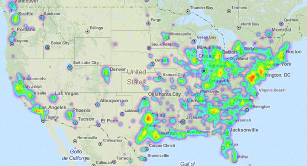
 The purpose of data visualization is to put information into a format that is easy to comprehend by the human brain. One way to visualize data is through color. Color is a very effective way to convey changes in data. While a random color palette is good for representing categorical data. Continuous data, such as temperature, time, or population is better represented with a continuous color palette, such as a gradient.
Color Gradients
A color gradient is one very useful tool for representing changes in a continuous dataset. A properly chosen gradient will allow a viewer to quickly assess both small and large changes in data. Given that gradients are such a useful tool, it is handy to know how to generate a gradient.
A gradient is simply a range of colors determined by their position. For the purpose of this post I will just be covering one dimensional gradients, also known as axial gradients. Being one dimensional, the axial gradient is a simple linear interpolation of values between two points. Commonly, only two colors are interpolated between in axial gradient. Multiple color gradients also exist. For example, the rainbow gradient displays the entire rgb color range (given equal brightness and saturation).
The Math
Calculating a two color gradient is very easy. For two color axial gradients, it is necessary to project a percent to a range determined by each of the components of an RGB color. For example, to build a gradient from the color rgb(42, 163, 90) to color rgb(207, 74, 33) there will be three different interpolations. The red component will be interpolated from 42 to 207. The green component will be interpolated from 163 to 74. The blue component will be interpolated from 90 to 33.
My previous post, “Range Mapping and Projecting Values”, covers all the math needed to interpolate between ranges. To recap, given an input value from 0 to 1 and an output range from red component 42 to red component 207 (1 byte color) the following equation can be used to get the projected value:
Given that our input range is clamped to the range 0 to 1, it is possible to simplify the equation to:
The Code
To leverage the code developed for the, “Range Mapping and Projecting Values” post, it is convenient to simply use the scale_value function to interpolate each color component independently. This allows the gradient_value function to be reduced to just a few lines, with each RGB color component being mapped from a range of 0 to 1 to the range of from_color.(r/g/b) to to_color.(r/g/b)
#include "range_map.hpp"

class rgb
{
public:
	using value_type = uint8_t;
	value_type r, g, b;
};

inline rgb gradient_value(const double_t value, const rgb & from_color, const rgb & to_color)
{
	using namespace range_map;
	return {
		scale_value(value, 0.0, 1.0, from_color.r, to_color.r),
		scale_value(value, 0.0, 1.0, from_color.g, to_color.g),
		scale_value(value, 0.0, 1.0, from_color.b, to_color.b) };
}
Optimizations
It it would be handy to leverage the equation simplification from above to reduce unnecessary processing and reduce the number of parameters needed when using using a clamped percentage. So the following code was developed and added to the range_map.hpp header:
//scales 'value' from the range 0.0/1.0 to the range 'lowestTo'/'highestTo'
template <class _TT,
class = typename std::enable_if<std::is_arithmetic<_TT>::value>::type>
	_TT scale_value(const double_t value, const _TT lowestTo, const _TT highestTo)
{
	if (value <= 0.0)
		return lowestTo;
	if (value >= 1.0)
		return highestTo;

	//scale by half to account for negative and positive range being too large to represent
	const auto && tHLF = [](_TT v){ return v / long double(2.0); };

	auto scaledOffsetResult = (tHLF(highestTo) - tHLF(lowestTo)) * value;
	return (_TT)(scaledOffsetResult + lowestTo + scaledOffsetResult); //seperated to prevent overflow
}
Now the gradient code can be simplified:
#include "markdown.hpp"
#include "range_map.hpp"

class rgb
{
public:
	using value_type = uint8_t;
	value_type r, g, b;
};

inline rgb gradient_value(const double_t value, const rgb & from_color, const rgb & to_color)
{
	using namespace range_map;
	return {
		scale_value(value, from_color.r, to_color.r),
		scale_value(value, from_color.g, to_color.g),
		scale_value(value, from_color.b, to_color.b) };
}

int main()
{
	using namespace markdown;

	ostream << table_header("cccc", "Transition1", "Transition2", "Transition3", "Transition4");
	for (int i = 0; i <= 10; ++i)
	{
		double_t v = (double_t)i / 10.0;
		auto make_cell = [](std::string clr)->std::string
		{return span(clr, color + "#ffffff", bg_color + clr); };

		ostream << table_row(
			make_cell(to_hex(gradient_value(v, { 255, 0, 0 }, { 0, 0, 0 }))),
			make_cell(to_hex(gradient_value(v, { 255, 255, 255 }, { 0, 0, 0 }))),
			make_cell(to_hex(gradient_value(v, { 0, 0, 0 }, { 255, 255, 255 }))),
			make_cell(to_hex(gradient_value(v, { 42, 163, 90 }, { 207, 74, 33 }))));
	}
}
The Output
| Transition1 | Transition2 | Transition3 | Transition4 |
|---|---|---|---|
| #ff0000 | #ffffff | #000000 | #2aa35a |
| #e50000 | #e5e5e5 | #191919 | #3a9a54 |
| #cc0000 | #cccccc | #323232 | #4a914e |
| #b20000 | #b2b2b2 | #4c4c4c | #5b8848 |
| #990000 | #999999 | #656565 | #6b7f42 |
| #800000 | #808080 | #7f7f7f | #7c773d |
| #660000 | #666666 | #989898 | #8c6e37 |
| #4d0000 | #4d4d4d | #b1b1b1 | #9c6531 |
| #330000 | #333333 | #cbcbcb | #ad5c2b |
| #1a0000 | #1a1a1a | #e4e4e4 | #bd5325 |
| #000000 | #000000 | #ffffff | #cf4a21 |
There are no tricks or gotcha’s with this code, all the work is performed in the scale_value function. In part 2 on gradients, I will cover another axial gradient and also create some fun test cases for the new functionality.